Using the GSN Composer as a Web-based Modular Synthesizer
The GSN Composer is a free web-based visual programming environment in which inputs and outputs of ready-made nodes are connected to generate an executable data-flow graph. The GSN Composer provides several audio processing nodes that are intended to be used together to generate sounds or music. Internally, these nodes use the Web Audio API for stream-based audio processing and the Web MIDI API to support external MIDI hardware. While Web Audio is implemented by most modern browsers, Web MIDI is currently only usable in Google Chrome or Microsoft Edge (Chromium version).
This tutorial introduces the most important nodes for stream-based audio processing. With these nodes you can build very different kind of synthesizers. We will provide examples for subtractive synthesis, additive synthesis, FM synthesis, wavetable synthesis and sample-based synthesis in the text below.
If you are new to the GSN Composer, you might want to start with the general Getting Started page before following the tutorial on this page.
Signal vs. Stream
The GSN Composer has two different data nodes that can be used for audio:
- SignalProcessing.
Data. Signal - AudioProcessing.
Data. Stream
A signal data node contains an array of floating-point values that can be interpreted as a mono track of audio data. The signal processing section within the create dialog contains many compute nodes to manipulate a signal data node. Signals can also be loaded from a WAV file and played back as an audio track, which is demonstrated in the Play Audio File example.
However, signal data nodes are not suitable for real-time audio manipulation because when any part of the signal is changed, the complete signal is marked as updated, the node graph is re-evaluated, and the audio playback of the signal starts again at the beginning.
Thus, if live real-time audio interaction is required, you need to work with the stream-based audio processing nodes. Stream data nodes do not directly contain any audio data. Instead they contain configuration information that defines which nodes of the Web Audio API should be instantiated and how they are connected. The Web Audio API performs stream processing in a separate thread independent from the main UI thread of the browser, which is essential for real-time performance. Therefore, the audio processing is also independent from the speed of the graph evaluation and visual update rate of the GSN Composer interface. Interactions, such as triggered midi notes or midi control changes, are immediately evaluated (not only when the graph of the GSN Composer is re-evaluated), which is essential for direct control via real and virtual midi devices.
To convert a signal into an audio stream use the AudioBuffer node that is described next.
AudioProcessing.Generate.AudioBuffer
The AudioBuffer node of the GSN Composer is mainly a wrapper for the AudioBufferSourceNode
of the Web Audio API. A signal connected to the input slot is moved as an audio asset over the thread boundary of the
Web Audio API and can be played back as an audio stream. The output stream can be connected to other stream-based audio processing nodes of the GSN Composer. Thereby, it is essential that
the audio routing graph terminates in a stream destination node, such as AudioProcessing.
The other input slots of the AudioBuffer node of the GSN Composer control different aspects of the streaming output. The speed factor and detune slots control the playback speed. The gain slot provides a multiplicative factor for the amplitude. When follow note is set to true, a triggered midi note affects the playback speed when used in combination with an instrument. Similarly, when velocity is set to true, the velocity of a triggered midi note affects the gain of the output.
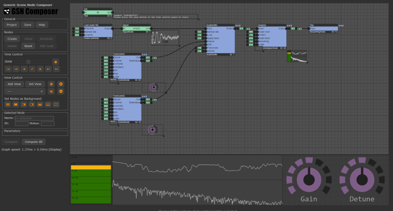
In the example below, an AudioBuffer node is used for stream-based audio playback of a loaded signal. During playback, the gain and detune parameter of the AudioBuffer node can be changed interactively via the provided knobs. If you have a hardware MIDI controller connected (and you are using Google Chrome) you should be also able to change the gain via the main volume controller and the detune parameter via the pitch bend controller.
AudioProcessing.Generate.Oscillator
The oscillator node of the GSN Composer is a wrapper for the OscillatorNode of the Web Audio API. The type input slot selects the shape of the periodic waveform: sine, square, sawtooth, or triangle.

The frequency allows to set the oscillator frequency in Hz, which defining how often the periodic waveform is repeated per second. The default value is 440 Hz, which is standardized as the note A above middle C (standard pitch). Oscillator are often used as sound sources in synthesizers. When the oscillator is used in combination with an instrument and follow note is set to true, the instrument will offset the oscillator's frequency according to the currently played note of a MIDI device. In contrast, the pitch slot is an option to offset the frequency of the oscillator, which is not effected by the currently played note. The pitch offset is specified in cents (one cent is 1/100th of a semitone).
The gain slot provides a multiplicative factor for the amplitude. When the oscillator is used in combination with an instrument and velocity is set to true, the velocity of a triggered midi note is used as an additional multiplicative factor for the gain.
The phase slot allows setting the oscillator's phase in range [0.0, 1.0] defining a small delay that is applied when the note is triggered. A phase of 0.0 means no phase offset (no delay) and a phase value of 1.0 means a delay of a complete period.
As an example, let's start with the most simple setup. A single oscillator is connected via an analyser to the play destination node. You can try to change the type, frequency, and amplitude and check with the analyser if the oscillator reacts as expected:

Now, we add a second oscillator that is detuned by 4 cents and merge the two output streams. Merging two audio streams simply adds the samples from both streams. Because both oscillators have slightly different frequencies, the superposition produces an interference pattern. The slower oscillator requires more time for one period and therefore the overlap of both waves shifts over time. Therefore, the two waves smoothly alternate between doubling their amplitude and canceling each other out:

AudioProcessing.Generate.LFO
A low-frequency oscillator (LFO) is a slowly varying oscillator that is typically used as a modulator of certain parameters of other audio nodes, e.g., modulating the amplitude generates a tremolo effect, modulating the pitch produces a vibrato effect, and modulating the filter cut-off frequency causes a ripple effect. In the GSN Composer, there is no major difference between an Oscillator node (described above) and a LFO node because both are wrappers for the OscillatorNode of the Web Audio API. The only difference is the smaller default frequency of 5 Hz. Furthermore, frequency and gain are not effected by the currently played note if the LFO is used within an instrument. When the LFO is used within an instrument and the retrigger parameter is set to true, a separate LFO is created and retriggered with every note. Otherwise, a conjoined LFO is used for all notes.
In the following example, the output stream of a LFO is connected to the detune input slot of a regular oscillator. Because the amplitude of the LFO is set to 1200.0, the detuned parameter of the regular oscillator is modulated by ±1200.0 cents (corresponding to ±12 semitones). Feel free to experiment a bit with this example: You could try to change the type and frequency of the LFO and observe the effect; or you could connect another LFO to the gain slot of the regular oscillator; or you let another LFO manipulate the parameters of the LFO, etc.

AudioProcessing.Instrument.Instrument
The instrument node of the GSN Composer is essential for triggering the playback of an audio graph with a real or virtual MIDI controller. Real hardware MIDI controllers are supported via the Web MIDI API, which is currently only usable in Google Chrome or Microsoft Edge (Chromium version).
For each note triggered by the MIDI controller, an instance of the complete upstream audio graph is created. Thereby, the instrument node adapts the frequency of every Oscillator and the speed factor of every AudioBuffer node in the upstream graph according to the currently played MIDI note. The reference slot sets the reference note for which the upstream graph was created. The default reference is the MIDI note A3 corresponding to a frequency of $f_{\tiny \mbox{ref}}=$ 440 Hz, which is standardized as the note A above middle C (standard pitch).
When a MIDI note with frequency $f_{\tiny \mbox{note}}$ is triggered, the output frequency $f_{\tiny \mbox{out}}$ of each oscillator with a selected frequency $f_{\tiny \mbox{sel}}$ is changed to:
The channel slot of the instrument node defines the MIDI channel to which the instrument is listening. When the value is set to -1 (the default) the instrument reacts to all midi channels.
If the polyphonic input parameter is set to true, the instrument can play multiple notes at once. For example, if three different MIDI notes are simultaneously played, three instances of the upstream graph are created, each with adapted oscillator frequencies and audio buffer speeds. The resulting three output streams are added and produce the output stream of the instrument node. If polyphonic is set to false, the playback of the current note is stopped, once a new note is triggered.
Typically, the playback of a note should be stopped if the MIDI controller sends a note off message. However, for some instruments, such as drums, an audio sample should continue playing until its end or until the same drum is triggered again. This can be achieved by setting the ignore off slot to true.
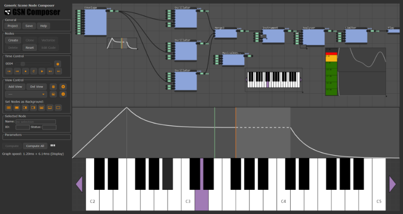
The example below demonstrates a simplistic instrument build from three oscillators. It can be triggered with a virtual or real MIDI controller.
Oscillator 1 and 2 have a frequency $f_{\tiny \mbox{sel}}$ of 440 Hz. Oscillator 3 a frequency $f_{\tiny \mbox{sel}}$ of 220 Hz. Oscillator 2 is detuned by 4 cents.
The reference note selected for the instrument is the MIDI note A3 corresponding to a frequency of $f_{\tiny \mbox{ref}}=$ 440 Hz.
Let us assume the MIDI controller triggers the node A4, which is one octave higher than the reference and corresponds to $f_{\tiny \mbox{note}}=$ 880 Hz.
The instrument would generate an instance of the upstream audio graph (which are the three oscillators and the merge node in this example) and would change the frequency of
oscillator 1 and 2 from 440 Hz to $f_{\tiny \mbox{out}}=$ 880 Hz. The detune value of 4 cents for oscillator 2 is unaffected.
For oscillator 3 the instruments adapts the frequency from 220 Hz to $f_{\tiny \mbox{out}}=$ 440 Hz.
If multiple MIDI notes are played simultaneously and polyphonic is set to true,
a separate instance of the upstream graph is created for each note. The contributions from each instance are added. This may cause clipping, if the sum
is outside of the allowed range between -1.0 and 1.0. To avoid clipping a dynamic range limiter is added to the audio graph.

An obvious problem of the above example are the popping sounds that occur when a note is released and the oscillators are suddenly turned off. This problem can be solved with an envelope node that is introduced next.
AudioProcessing.Generate.Envelope
This node generates an classical ADSR envelope (ADSR = Attack, Decay, Sustain, Release) and is typically used in combination with the instrument node described above. When the instrument node receives a note-on message from a real or virtual MIDI controller, an individual note envelope is started and can be used to modulate certain parameters of other audio nodes over time.

Attack: After a note-on message the attack phase starts. The attack input slot sets the length of the attack in seconds. The attack envelope starts at 0.0 and reaches the value specified by the attack level parameter after the specified time. The shape of the attack curve can be linear or exponential, which is selectable via the attack type slot.
Decay: After the attack phase follows the decay phase. The decay input selects the length of the decay in seconds and decay type the shape of the envelope curve. The decay part of the envelope starts at the value specified by attack level and reaches the the value define by sustain level after the specified time.
Sustain: After the decay phase follows the sustain phase. During the sustain phase the envelope's amplitude is kept constant. Thereby, the constant sustain amplitude is defined by the sustain level value. The sustain phase does not have a predefined duration. It continues endlessly until a note-off message from the MIDI controller is received.
Release: After a note-off message from the MIDI controller, the release phase starts. This is always the case even if the time for the attack phase or decay phase has not passed and the sustain phase was not reached. If the sustain phase was reached, the envelope of the decay phase starts at the sustain level and goes towards zero. The release input selects the length of the release phase in seconds and release type the shape of the envelope curve. If the sustain phase is not reached when the note-off message occurs, the release envelope starts from the current amplitude value and goes towards zero. Unfortunately, the required Web Audio cancelAndHoldAtTime function is not supported by all browsers (Google Chrome works).
The complete envelope is multiplied with the value selected via the amplitude parameter. The amplitude can be freely chosen (it can also be negative). For example, if the amplitude is 1000.0 and the sustain level is 0.6, the envelope value would be 600.0 during the sustain phase.
Besides the core ADSR envelope functionality, the delay input slots allows specifying a delay in seconds that is applied between the note-on message and the start of the attack. This is useful if certain aspects of a sound require a later onset.
The envelope node visualizes the shape of the applied envelope. Thereby, the current envelope positions of the played notes are displayed by vertical colored lines. This visualization can be helpful while manipulating the envelope's parameters to produce a desired effect.
As a first example, we fix the graph from above, where an instrument was build from three oscillators. An envelope node is added and its output is connected to the gain inputs of all three oscillators. Because of the smooth attack and release transitions the "pop" artifacts are removed.
In the second example, a kick drum sound is synthesized by using an ADSR envelope for pitch and amplitude modulation of a triangle wave.

The triangle oscillator has a high frequency in the beginning that drops down very fast by 4 octaves (4800 cents). This is achieved with an envelope on the pitch slot of the oscillator with the following parameters:
- Amplitude: -4800.0 (cents)
- Attack: 0.0015 seconds, Attack level: 1.0
- Decay: 0.8 seconds, Sustain level: 1.2
- Release: 0.0 seconds
Note, that the amplitude parameter is set to to a negative value to achieve the negative pitch modulation. The attack time is very fast (1.5 milliseconds). This is very challenging for some browsers which is why the latency in the instrument is raised from the usual 0.010 to 0.030 seconds (30 milliseconds) in order to give the browser a larger head start. The sustain level is even larger than the attack level, which means that the pitch is further decreased in the decay phase. After the decay phase the pitch is -4800.0 cents ∗ 1.2 = -5760.0 cents. The release time is set to 0.0. The release phase is never reached anyway because the ignore off slot is set to true in the instrument. This makes sense because a drum should always sound the same, independent from the duration of the MIDI note.
The amplitude envelope is connected to the gain slot of the oscillator and has the following parameters:
- Amplitude: 1.0
- Attack: 0.0 seconds, Attack level: 1.0
- Decay: 0.5 seconds, Sustain level: 0.0
- Release: 0.0 seconds
An attack time of 0.0 seconds means that no attack ramp is used at all. This is important for a drum sound because otherwise the initial punch is dampened. The sustain level is set to 0.0 because the release phase can not take care of turning the sound off (as it is never reached).
The advantage of a synthesized kick drum over playing a kick drum sample is that it can be freely customized. For example, you could change from a triangle wave to a sine wave, change the envelopes, use multiple oscillators with different wave forms, add noise, etc.
AudioProcessing.Instrument.InstrumentMulti
The InstrumentMulti node is an extension of the regular Instrument node (described above) and is essential for building instruments from multiple audio samples or synthesized sounds. It allows keyboard splits and velocity-dependent sound selection.
The key difference to the Instrument node is that the InstrumentMulti node takes a vector of input audio streams instead of a single stream. Which audio stream from the input vector is selected to produce the sound for a triggered MIDI note depends on the configuration in the mapping input slot. For each audio stream in the input vector, the mapping parameter text should contain one line with the following syntax:
{NoteRef} > {NoteStart}--[NoteEnd] : [VelStart]--[VelEnd]
This is best explained with several examples. In a first example, we build a sample player. To this end, the InstrumentMulti node is used together with an AudioBuffer node to create a piano instrument from 14 audio samples.

The created piano has 7 octaves: C1 to B7. We load 14 audio samples and pass them as a vector into the AudioBuffer node, which creates a vector of 14 audio streams. For each octave we provide the D and the A note and configure the InstrumentMulti node to synthesize the intermediate notes by resampling. As the vector comprises of 14 audio stream, the mapping text has 14 lines:
D1 > C1--F1
A1 > F#1--B1
D2 > C2--F2
A2 > F#2--B2
D3 > C3--F3
A3 > F#3--B3
D4 > C4--F4
A4 > F#4--B4
D5 > C5--F5
A5 > F#5--B5
D6 > C6--F6
A6 > F#6--B6
D7 > C7--F7
A7 > F#7--B7
which means that the first audio stream has a reference note of D1 and maps to the range C1 to F1 on the MIDI keyboard, the second audio stream has a reference note of A1 und maps to the range F#1 to B1, and so on.
In the second example, velocity sensitivity is demonstrated.
In order to have three very recognizable sounds dependent on the velocity of a triggered MIDI key, three oscillators with three different waveforms (sine, triangle, and square) are employed and mapped to different velocity ranges:
A3 > C-2--G8 : 000--079
A3 > C-2--G8 : 080--103
A3 > C-2--G8 : 104--127
which means that for any MIDI controller key (from the lowest possible note C-2 to the highest possible G8) triggered with a velocity in the range 0 to 79 the first audio stream is used (sine wave), for a velocity in range 80 to 103 the second audio stream (triangle wave), and from 104 to 127 the third (square wave). The reference note is A3 because the oscillators are tuned to 440 Hz (standard pitch).
AudioProcessing.Effect.BiquadFilter
The biquad filter node is a wrapper for the
BiquadFilterNode of the Web Audio API.
It can be used to filter an audio stream with different filter types that are selectable with the type parameter and
are listed
in the following:
Type = 0: Lowpass: When the biquad filter is set to this type, a lowpass IIR filter with 12dB/octave rolloff is realized. Such a lowpass filter is commonly used for sound design. A steeper 24 dB/octave attenuation can be achieved with two biquad filters connected in series. The frequency and pitch input slots define the cut-off frequency, and the Q factor slot the filter's resonance (in dB) around the cutoff frequency. The gain slot is not used for this type of filter. The figure below (left) shows the frequency response of the lowpass biquad filter for different parameters.
Type = 1: Highpass: When the biquad filter is set to this type, a highpass IIR filter with 12dB/octave rolloff is realized. The frequency and pitch input slots define the cut-off frequency, and the Q factor slot the filter's resonance (in dB) around the cutoff frequency. The gain slot is not used for this type of filter. The figure below (center) shows the frequency response of the highpass biquad filter for different parameters.
Type = 2: Bandpass: When the biquad filter is set to this type, a bandpass IIR filter is realized. The frequency and pitch input slots define the passband's center frequency, and the Q factor controls the width of the passband. A higher Q factor results in a more narrow passband. The gain slot is not used for this type of filter. The figure below (right) shows the frequency response of the bandpass biquad filter for different parameters.


Type = 3: Lowshelf: When the biquad filter is set to this type, a lowshelf IIR filter is realized. The frequency and pitch input slots define the frequency below which a change to the spectrum is made, and the gain defines the amount of change in dB. The Q factor slot is not used for this type of filter. The figure below (left) shows the frequency response of the lowshelf biquad filter for different parameters.
Type = 4: Highshelf: When the biquad filter is set to this type, a highshelf IIR filter is realized. The frequency and pitch input slots define the frequency above which a change to the spectrum is made, and the gain defines the amount of change in dB. The Q factor slot is not used for this type of filter. The figure below (right) shows the frequency response of the highshelf biquad filter for different parameters.


Type = 5: Peaking: When the biquad filter is set to this type, a peaking IIR filter is realized. The frequency and pitch input slots define the filter's center frequency, and the gain the amount of change in dB. The Q factor slot controls the width of the changed frequency band. A higher Q factor results in a more narrow band. The figures below show the frequency response of the peaking biquad filter for different parameters.


Type = 6: Notch: When the biquad filter is set to this type, a notch IIR filter is realized. The frequency and pitch input slots define the center frequency of the rejection band, and the Q factor controls the width of the band. A higher Q factor results in a more narrow band. The gain slot is not used for this type of filter. The figure below (left) shows the frequency response of the notch biquad filter for different parameters.
Type = 7: Allpass: When the biquad filter is set to this type, an allpass IIR filter is realized that does not affect the amplitude of the spectrum but only its phase. The frequency and pitch input slots define the center frequency of the phase transition, and the Q factor controls the sharpness of the transition. A higher Q factor results in a sharper phase transition. The gain slot is not used for this type of filter. The figure below (right) shows the phase response of the allpass biquad filter for different parameters.


The influence of a biquad filter on an audio stream can be sonified by feeding white noise to its input. White noise has a flat spectral density and, consequently, most filter settings will result in a audible effect. This is demonstrated in the following example:

Subtractive Synthesis
At this point of the tutorial, we have introduced all necessary nodes to perform subtractive synthesis of sounds.
The general idea of subtractive synthesis is to start off with a wave that contains many different frequencies in its spectrum and attenuate some frequencies with a filter to create the desired sound.
In the image below, the spectra for a sine, square, sawtooth, and triangle wave are shown. The x-axis of the spectra is normalized to the fundamental frequency of the played note. A sine wave only contains the fundamental frequency. Thus, it is not a good candidate for subtractive synthesis because there is not much to remove. In contrast, the square wave additionally contains all the odd harmonics of the fundamental. The sawtooth wave contains the fundamental and all harmonics (odd and even ones). The triangle wave is similar to the square wave and contains the fundament and all odd harmonics but the amplitude of the harmonics gets comparably smaller with higher frequency.

To build a subtractive synthesizer we should limit the number of employed nodes. If many nodes are used, the synthesizer typically gets more versatile but this comes at the cost of computational effort and the number of parameters that needs to be tweaked.
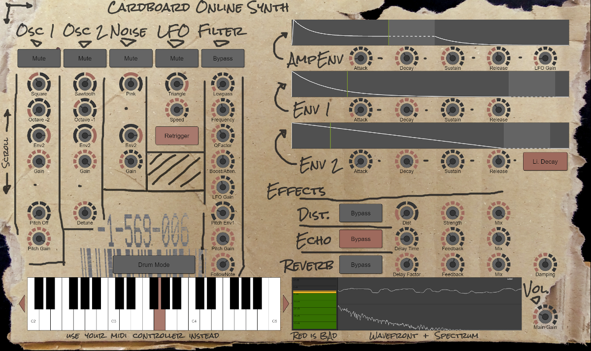
The subtractive synthesizer in the following example is build from two oscillators, one noise generator, two chained biquad filters, an LFO, and three ADSR envelopes. Its schematic is shown below.

The sound for each note that is played with this synthesizer emerges from three sound sources: oscillator 1, oscillator 2, and a noise generator. The output of these sound sources is added and fed into a chain of two biquad filters. The two biquad filters are connected in series in order to achieve a 24 dB/octave filter attenuation. All filter parameters are used conjointly by both filters. Afterwards, an ADSR envelope is applied to the output amplitude. The LFO can be used in two ways: Firstly, it can be added via the "Amp. LFO Gain" to the amplitude, which creates a tremolo effect. Secondly, it can be added via the "Filter. LFO Gain" to the pitch/detune slots of both biquad filters, which creates a ripple effect. Additionally, we have envelopes 1 and 2, which are freely assignable for different tasks. In total there are 6 variants: off (a constant audio stream with amplitude 0.0), envelope 1, negative envelope 1, envelope 2, negative envelope 2, and full (a constant audio stream with amplitude 1.0). Any of these 6 variants can be selected for the gain of the three sound sources, or the pitch/detune of oscillator 1, or via the "Filter. Pitch Gain" for the pitch/detune slots of both biquad filters.
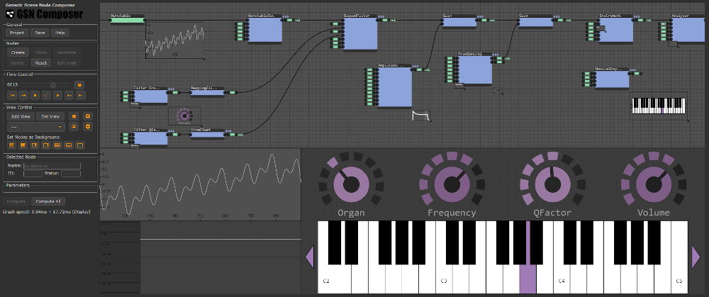
After we have created the basic nodes for this synthesizer, we can create a user interface that exposes the important parameters. Furthermore, we insert a distortion, delay, and reverb node after the instrument node. Creating the user interface is a bit tedious as there are approx. 60 parameters in total. Most parameters are exposed as knobs and for each knob a suitable parameter range must be selected. Here is the final result:
If you open the example, there are several presets available that demonstrate the capabilites of this subtractive synthesizer. If you are using Chrome you can also use a hardware MIDI controller. The complete node graph that created the example above is available here.
AudioProcessing.Generate.PhaseModOsc (for FM Synthesis)
The PhaseModOsc node is a special variant of the oscillator node with a stream input for the phase offset. This node is useful as an operator in FM synthesis. Though it is called frequency modulation (FM) synthesis, in fact, most synthesizers perform a phase modulation of a carrier signal, as it is explained here. Mathematically, if the carrier is a sine wave with frequency $f_c$ and $\mathrm{m}(t)$ is the modulator function, we get:
For FM synthesis, the frequency of the phase modulator $\mathrm{m}(t)$ is typically very fast. Often even faster than the frequency of the carrier. In this context, an important term in FM synthesis is the "ratio", which describes the relation of frequencies of the modulator and the carrier:
For harmonic sound (such as strings, leads, bass, pads, etc.) the ratio is typically formed by integer numbers (e.g., 4:1, 3:1, or 1:2). For metallic or bell-like sounds it can contain fractional values (e.g., 2.41 : 1). These ratios produce atonal and dissonant sounds that are difficult to generate with subtractive synthesis.
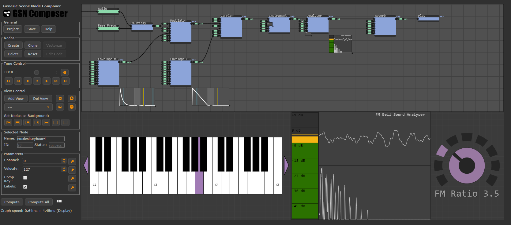
In the example below, a bell sound is synthesized, which is a classical example for FM synthesis. To this end, a sine modulator changes the phase offset of a sine carrier signal. The ratio of both oscillators is set to 3.5 : 1. Try changing the ratio via the knob. It will significantly change the sound of the bell.
AudioProcessing.Generate.WavetableOsc (for Wavetable Synthesis)
The idea of wavetable synthesis is to generate sounds by using periodic waveforms. Instead of generating these waveforms with a standard oscillator, the samples of the periodic waveform are precomputed (or are extracted from the recording of a real instrument) and are stored in a table. It is called a "table" but in fact it is simply an array of sample values. Thereby, each table contains exactly one complete period of the waveform. If the table content is played in a loop, the corresponding sound is created. Because these periodic waveforms can have arbritrary shapes, very different sounds can be produced.
In multiple wavetable synthesis several wavetable oscillators are used and time-varying crossfading or wavestacking is applied.
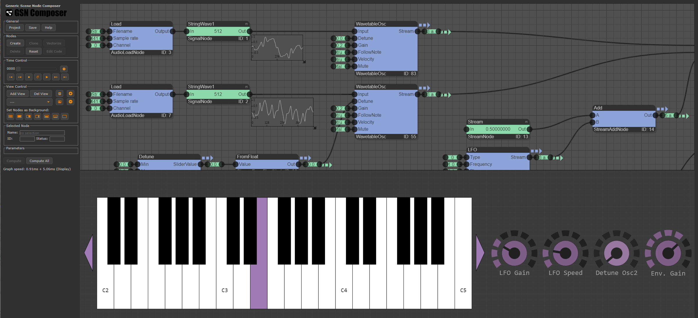
As a first example, we create an instrument from two wavetables that are extracted from the recording of a string ensemble. The crossfading of the two waveforms is modulated with an LFO.
The next example demonstrates how to combine a wavetable oscillator with a filter.
AudioProcessing.Generate.PeriodicWave (for Additive Synthesis)
The PeriodicWave node is the most versatile oscillator provided by the GSN Composer. It is a wrapper for the PeriodicWave node of the Web Audio API. Similar as the WavetableOsc (see above), it allows sound synthesis with arbitrary periodic waveforms. The advantage of the PeriodicWave node is that the resulting waveform is not detuned by resampling but by direct additive synthesis, which robustly avoids resampling artefacts (such as aliasing). The additive synthesis process is controlled by the real and imaginary signal slots, which are connected with input signals containing weighting factors for the additive cosine and sine functions. The resulting wavefront is given by:
where $a[u]$ represents the real input signal and $b[u]$ the imaginary input signal. The output wavefront is normalized to the amplitude selected by the gain input slot. The other slots are well known from the other oscillators described above. Most importantly, the PeriodicWave node has a phase mod slot to modulate the phase offset, which means that this oscillator can be used as an operator in FM synthesis as well.
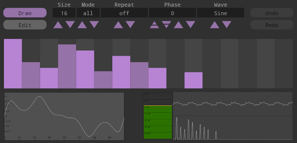
In the following example, we create the real and imaginary input signals for the PeriodicWave node using the HarmonicWave helper node, which allows interactive sketching of the harmonic components.
AudioProcessing.Generate.PeriodicFour
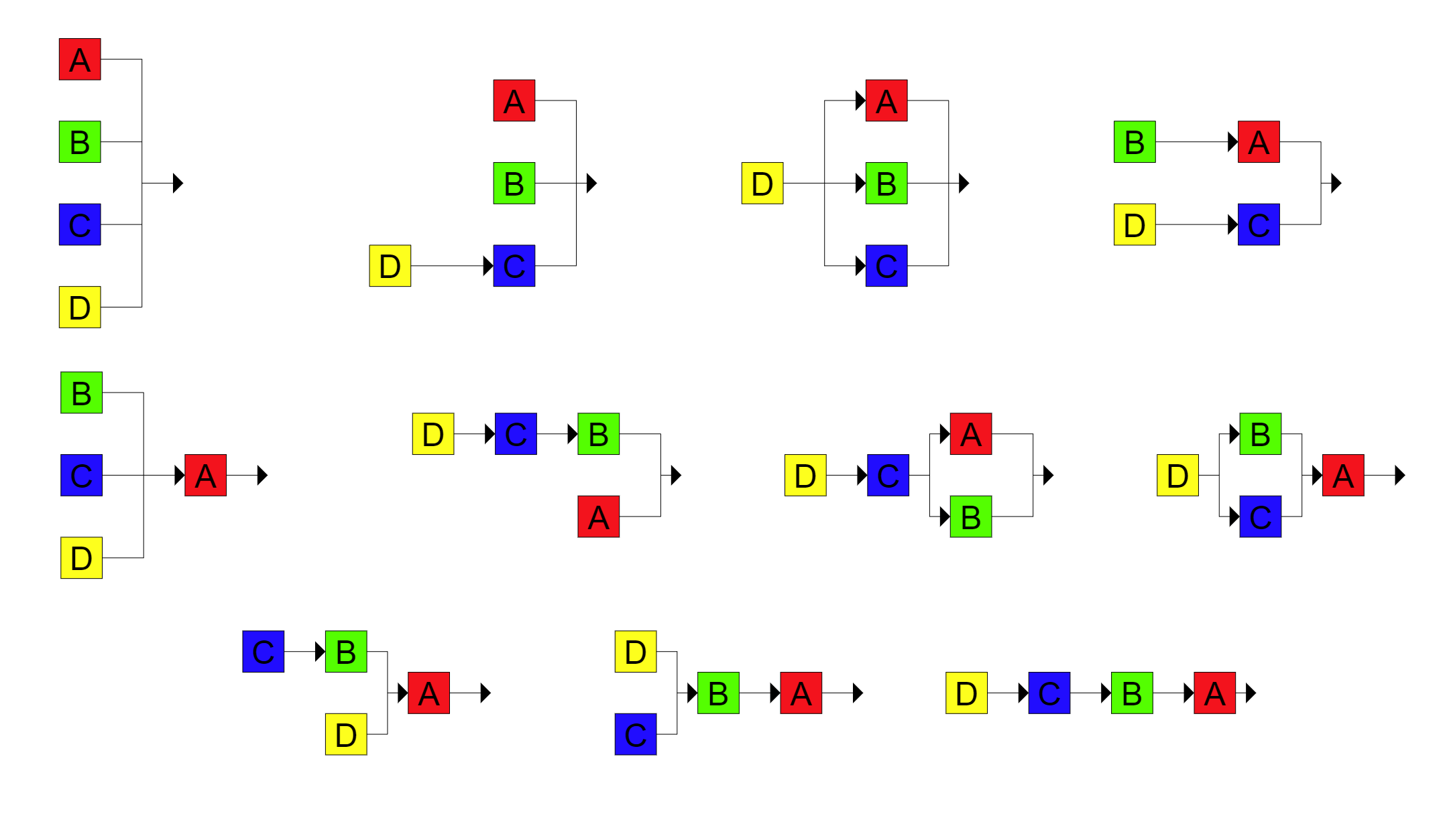
The PeriodicFour node contains a ready-made packaging of four PeriodicWave nodes (see above). These four PeriodicWave oscillators are labeled A, B, C, and D. Internally, the four oscillators are connected in different configurations and can be used as operators for FM synthesis. This means that the output of one oscillator modulates the phase of the next oscillator in the chain. In FM synthesis, the different configurations are typically called "algorithms". A total of 11 different algorithms are available that are shown below and can be selected via the algorithm input slot.
Furthermore, the output of each oscillator can be used as an additional modulator for its own phase, creating a feedback loop. Each oscillator has an feedback input slot that defines the gain of the feedback loop. A feedback value of 0.0 means that no feedback is used.
For each oscillator, the velocity input slot defines a weighting factor in the range [-1, 1] for the velocity. This weighting factor is multiplied by the velocity of a triggered MIDI note. The resulting product is used as a multiplicative factor for the oscillator's gain.
The other input slots are already known from the PeriodicWave node described above.
Further Topics and User Feedback
The GSN Composer also provides a step sequencer node that allows you to compose complete songs with multiple instruments by playing, editing, or recording MIDI messages.
The GSN Composer is constantly evolving and user feedback is very welcome. Please use the contact form or visit the forum on Reddit if you have questions or suggestions for improvement.