ImageProcessing.Compute.Filter.Edge
- Type = 0: Sobel
- Type = 1: SobelXY
- Type = 2: Prewitt
- Type = 3: PrewittXY
Sobel Filter
If "SobelXY" is selected, the image is convolved with 2D Sobel kernels. The half-size input slot selects the size of the kernel. For a half-size $h$ of 1 (which is the default) the resulting kernel size is $k= 2\,h + 1 = 3$, which results in the widely used 3 x 3 Sobel kernels in x- and y-direction:
$\mathtt{S}_x = \frac{1}{8}\begin{bmatrix}1 & 0 & -1\\
2 & 0 & -2\\
1 & 0& -1 \end{bmatrix} \quad \quad
\mathtt{S}_y = \frac{1}{8}\begin{bmatrix}\begin{array}{rr} 1 & 2 & 1\\
0 & 0 & 0\\
-1 & -2& -1 \end{array} \end{bmatrix} $
Both 3 x 3 Sobel kernels can be separated into a derivative kernel and a perpendicular binomial smoothing kernel:
$\mathtt{S}_x = \frac{1}{8} \begin{bmatrix}1 & 0 & -1\\
2 & 0 & -2\\
1 & 0& -1 \end{bmatrix} = \frac{1}{4}\begin{bmatrix}1\\
2\\
1 \end{bmatrix} \,\, \ast \,\, \frac{1}{2}\begin{bmatrix}1 & 0 & -1\\ \end{bmatrix}$
$\mathtt{S}_y =
\frac{1}{8} \begin{bmatrix}\begin{array}{rr}
1 & 2 & 1\\
0 & 0 & 0\\
-1 & -2& -1 \end{array}\end{bmatrix} = \frac{1}{4}\begin{bmatrix}1 & 2 & 1\\ \end{bmatrix} \,\, \ast \,\, \frac{1}{2}\begin{bmatrix}\begin{array}{r}1\\
0\\
-1 \end{array}\end{bmatrix}$
For larger values of half-size the binomial smoothing kernel is increased but the derivative kernel remains the same size, e.g. for $h=2$
the 5 x 3 kernel for $\mathtt{S}_x$ and the 3 x 5 kernel for $\mathtt{S}_y$ are given by
$\mathtt{S}_x = \frac{1}{32}
\begin{bmatrix}1 & 0 & -1\\
4 & 0 & -4\\
6 & 0 & -6\\
4 & 0 & -4\\
1 & 0 & -1\\
\end{bmatrix} = \frac{1}{16}\begin{bmatrix}1 \\4\\ 6\\ 4\\ 1\\ \end{bmatrix} \,\, \ast \,\, \frac{1}{2}\begin{bmatrix}1 & 0 & -1\\ \end{bmatrix} $
$\mathtt{S}_y = \frac{1}{32}
\begin{bmatrix}\begin{array}{rr} 1 &4& 6&4& 1\\
0& 0 & 0 & 0 & 0 \\
-1 &-4& -6&-4& 1\\ \end{array}
\end{bmatrix} = \frac{1}{16}\begin{bmatrix}1 &4& 6&4& 1\\ \end{bmatrix} \,\, \ast \,\, \frac{1}{2}\begin{bmatrix}\begin{array}{r}1\\
0\\
-1 \end{array}\end{bmatrix}$
Note: Some other image processing applications apply smoothing in x- and y-direction for larger kernels. If a similar effect is required,
a blur node can be used as a pre-filter before a default 3 x 3 Sobel kernel is applied.
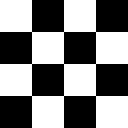
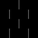
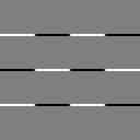
If the selected type is "SobelXY" and the input pixel values are in range [0.0, 1.0], the output pixels are in range [-0.5, 0.5]. Below is the output for
a black and white checkerboard input. As negative intensity values are clamped to zero when displayed, the output colors must be shifted by 0.5 to make the negative values visible.
| 
| 
| 
| 
|
| Input | X-Gradient from kernel $\mathtt{S}_x$ |
Y-Gradient from kernel $\mathtt{S}_y$ |
X-Gradient + 0.5 | Y-Gradient + 0.5 |
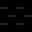
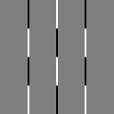
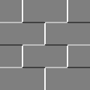
If the selected type is "Sobel" the magnitude and phase are computed from the x-gradient $\mathbf{g}_x$ and y-gradient $\mathbf{g}_y$ pixel values.
The magnitude $\mathbf{m}$ and phase $\mathbf{\theta}$ for each pixel are given by
$\mathbf{m} = \sqrt{\,\,\mathbf{g}_x^2 + \mathbf{g}_y^2} \quad , \quad \mathbf{\theta} = \DeclareMathOperator{\atantwo}{atan} \atantwo_2(\mathbf{g}_y, \mathbf{g}_x) \frac{2}{\pi} + 0.5 $
Here the phase is already shifted and scaled such that the resulting pixel values are in range [0.0, 1.0]. The images below show the output for a black and white checkerboard input.
|
| 
| 
|
| Input | Magnitude $\mathbf{m}$ | Phase $\mathbf{\theta}$ |
Prewitt Filter
If the selected type is "Prewitt" or "PrewittXY", the applied algorithms are very similar to the Sobel filter described above. The only difference is that the smoothing filter is a box filter. For example, the 3 x 3 kernels are given by:
$\mathtt{S}_x = \frac{1}{6} \begin{bmatrix}1 & 0 & -1\\
1 & 0 & -1\\
1 & 0& -1 \end{bmatrix} = \frac{1}{3}\begin{bmatrix}1\\
1\\
1 \end{bmatrix} \,\, \ast \,\, \frac{1}{2}\begin{bmatrix}1 & 0 & -1\\ \end{bmatrix}$
$\mathtt{S}_y =
\frac{1}{6} \begin{bmatrix}\begin{array}{rr}
1 & 1 & 1\\
0 & 0 & 0\\
-1 & -1& -1 \end{array}\end{bmatrix} = \frac{1}{3}\begin{bmatrix}1 & 1 & 1\\ \end{bmatrix} \,\, \ast \,\, \frac{1}{2}\begin{bmatrix}\begin{array}{r}1\\
0\\
-1 \end{array}\end{bmatrix}$
The example EdgeDetection demonstrates how to use this node for edge detection.